| Upwelling | Post-Upwelling | Winter | |
|---|---|---|---|
| Hubb's beaked whale | |||
| Oregon | 0.0000 (1430) | 0.0000 (493) | – (–) |
| Humboldt | 0.0000 (489) | 0.0010 (1048) | 0.0000 (308) |
| San Francisco | 0.0000 (960) | 0.0000 (688) | – (–) |
| Morro Bay | 0.0010 (2034) | 0.0000 (1353) | – (–) |
| Baird's beaked whale | |||
| Oregon | 0.0007 (1430) | 0.0000 (493) | – (–) |
| Humboldt | 0.0000 (489) | 0.0049 (1048) | 0.0033 (308) |
| San Francisco | 0.0031 (960) | 0.0176 (688) | – (–) |
| Morro Bay | 0.0069 (2034) | 0.0015 (1353) | – (–) |
| Stejneger's beaked whale | |||
| Oregon | 0.0000 (1430) | 0.0000 (493) | – (–) |
| Humboldt | 0.0000 (489) | 0.0010 (1048) | 0.0000 (308) |
| San Francisco | 0.0000 (960) | 0.0000 (688) | – (–) |
| Morro Bay | 0.0015 (2034) | 0.0000 (1353) | – (–) |
| Goose-beaked whale | |||
| Oregon | 0.0000 (1430) | 0.0000 (493) | – (–) |
| Humboldt | 0.0000 (489) | 0.0000 (1048) | 0.0000 (308) |
| San Francisco | 0.0147 (960) | 0.0250 (688) | – (–) |
| Morro Bay | 0.0947 (2034) | 0.0642 (1353) | – (–) |
Beaked Whales
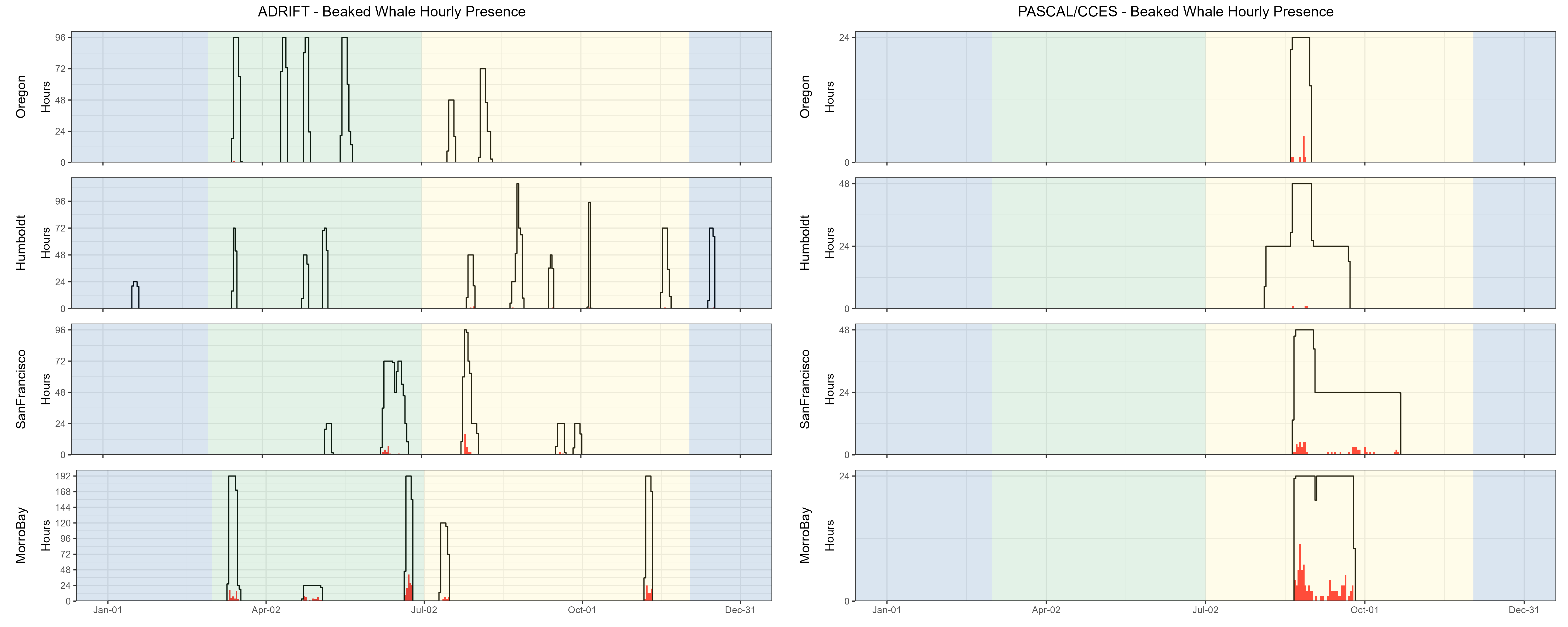
Detection of beaked whale species included: goose-beaked whales (Zc), Baird’s beaked whales (Bb, Berardius bairdii), Blainville’s beaked whales (Md, Mesoplodon densirostris), Stejneger’s beaked whales (Ms, M. stejnegeri), Hubb’s beaked whales (Mc, M. carlhubbsi, formerly BW37V), Cross Seamount Beaked Whale (BWC), and unidentified beaked whale BW43 (BW43, recently identified as M. ginkgodens, Mc, (Henderson et al., n.d.). Beaked whales were detected in all regions (Figure 1), and species detected in Adrift data included Baird’s beaked whales, Hubb’s beaked whales, Stejneger’s beaked whales, and goose-beaked whales (see table, right). Detection of beaked whales was higher in low latitude regions than in higher latitudes for the combined CCES and PASCAL surveys (Figure 1).
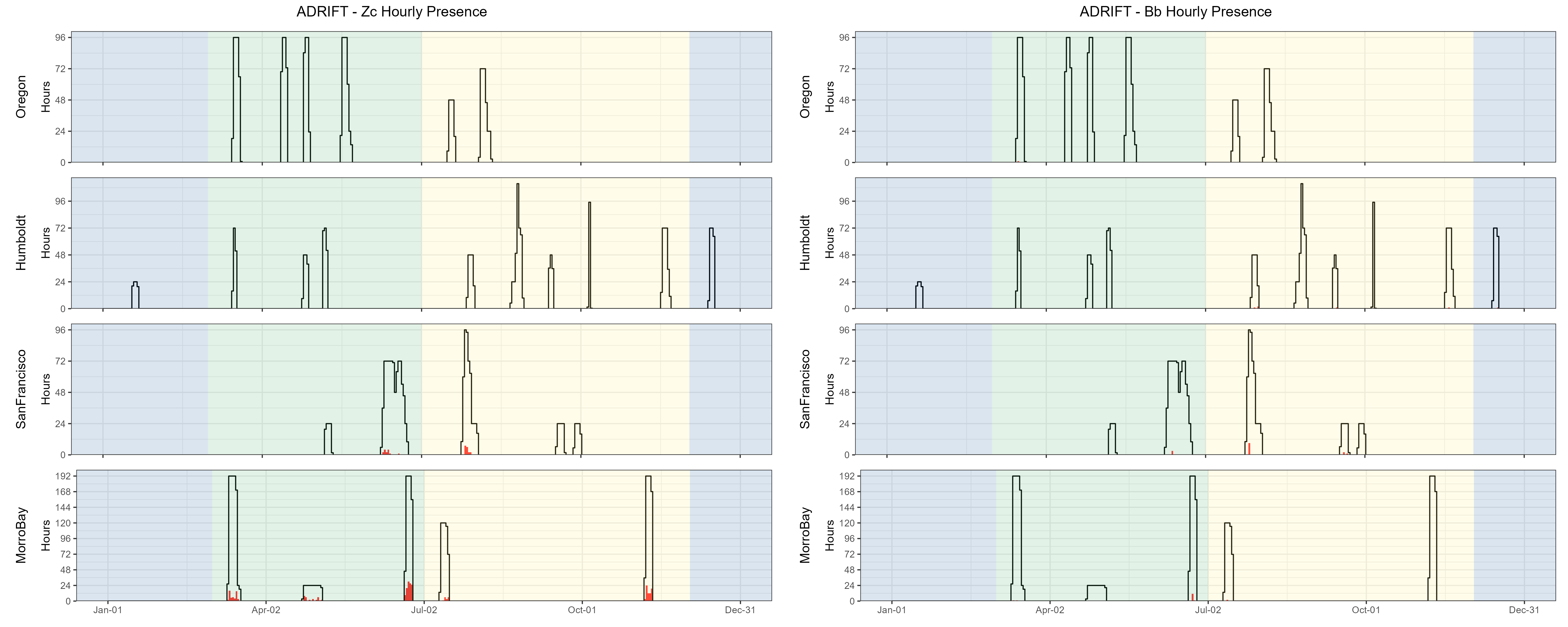
All beaked whale species were detected in Morro Bay, with relatively high probability of detection for goose-beaked whales (see table, right, and Figure 2). While goose-beaked whales were the most common species detected overall, there were no detections of this species in either Humboldt or Oregon study areas.
There had been no visual detection of beaked whales during the 30 years of annual ACCESS surveys offshore San Francisco (J. Roletto, pers. comm.).
The drifting recorders deployed during the ACCESS surveys detected both Baird’s and goose-beaked whales, suggesting that beaked whales do occur in and near the shipping lanes and the combined Greater Farallones and Cordell Bank National Marine Sanctuaries (Figure 2). The discrepancy in these detections is likely due to the typically poor sighting conditions in this region and the cryptic surfacing behavior of beaked whales. Future surveys in this region should consider passive acoustic monitoring with sufficient bandwidth to detect echolocating beaked whales.
Many of the beaked whale detections in Morro Bay occurred during times with large numbers of dolphin detections (see Contributors to Soundscape: [Acoustic Scene Morro Bay] 2022()https://sael-swfsc.github.io/Adrift/content/contributorsSS.html#fig-Adrift_MorroBay22_Seasons and Acoustic Scene Morro Bay 2023 for a visualization of this co-occurrence). Dolphins frequently occur in large schools with many animals echolocating simultaneously. It can be very difficult to identify beaked whales (smaller group sizes where fewer clicks are detected from each group) in these situations. The vertical hydrophone array allows for the estimation of bearing angles of incoming echolocation clicks. Beaked whales echolocate at depths below the vertical array, providing bearing angles > 90⁰ on the hydrophone array, while dolphins are typically above the array (bearing angles < 90⁰). By segregating the data based on bearing angle, we were able to identify groups of echolocating beaked whales during times where there were large numbers of echolocating dolphins. The co-occurrence of dolphins and beaked whales has not been previously reported, and it is unclear what may bring these species together. The likelihood of detecting beaked whales in these mixed species encounters would have been very low if recordings were collected from a single, seafloor sensor or from towed hydrophone arrays.
Detailed methods are provided in our Adrift Analysis Methods.
A protocol for estimating the density of goose-beaked whales from acoustic detections using drifting hydrophone recorders was established by (Barlow et al. 2022). We developed an open-source R package RoboJ (Robotic Jay) for these methods (see Data Sharing/Software). We explored automated event definition based on MTC (matched template classifier) scores and developed a process that identified every manually labeled event, but ultimately included an unacceptable number of false detections. The inclusion of a computer vision model was helpful for separating false detections; however, data processing times and classification rates were not acceptable. Current ideas to improve performance of automated event definition are discussed in Beaked Whale Analytical Tools. Data were prepared for future density estimation, but density estimates were not completed for Adrift or CCES survey data.
References
Barlow, Jay, Jeffrey E. Moore, Jennifer L. K. McCullough, and Emily T. Griffiths. 2022. “Acoustic-Based Estimates of Cuvier’s Beaked Whale (Ziphius Cavirostris) Density and Abundance Along the U.S. West Coast from Drifting Hydrophone Recorders.” Marine Mammal Science 38 (2): 517–38. https://doi.org/10.1111/mms.12872.
Henderson, E. Elizabeth, Lisa Ballance, Gustavo Cárdenas-Hinojosa, Jay Barlow, Annamaria I DeAngelis, Sergio Martinez, Craig Hayslip, et al. n.d. “First at-Sea Identifications of Gingko-Toothed Beaked Whale (Mesoplodon Gingkodens): Acoustics, Genetics, and Biological Observations Off Baja California, Mexico.” Marine Mammal Science In Prep.