Modeling Habitat Use

In order to consider passive acoustic data for population assessment of marine mammals, these methods must account for varying detection probabilities due to uncertainty in the source location and with changing background noise levels.

The clustered deployments off Morro Bay provide a test bed for evaluating the ability of drifting recorders to contribute to population assessment models. Mysticete calls can be detected on multiple instruments; however, localization of the sound source is limited by gaps in known sensor location (30 min GPS updates). As part of the exploratory analysis, we built a simulation of fin whale habitat use using regional density estimates, simplified propagation models and noise levels from one Morro Bay datasets. This simulation examined the potential spatial resolution of calls given the changing spacing of recorders throughout the deployment.

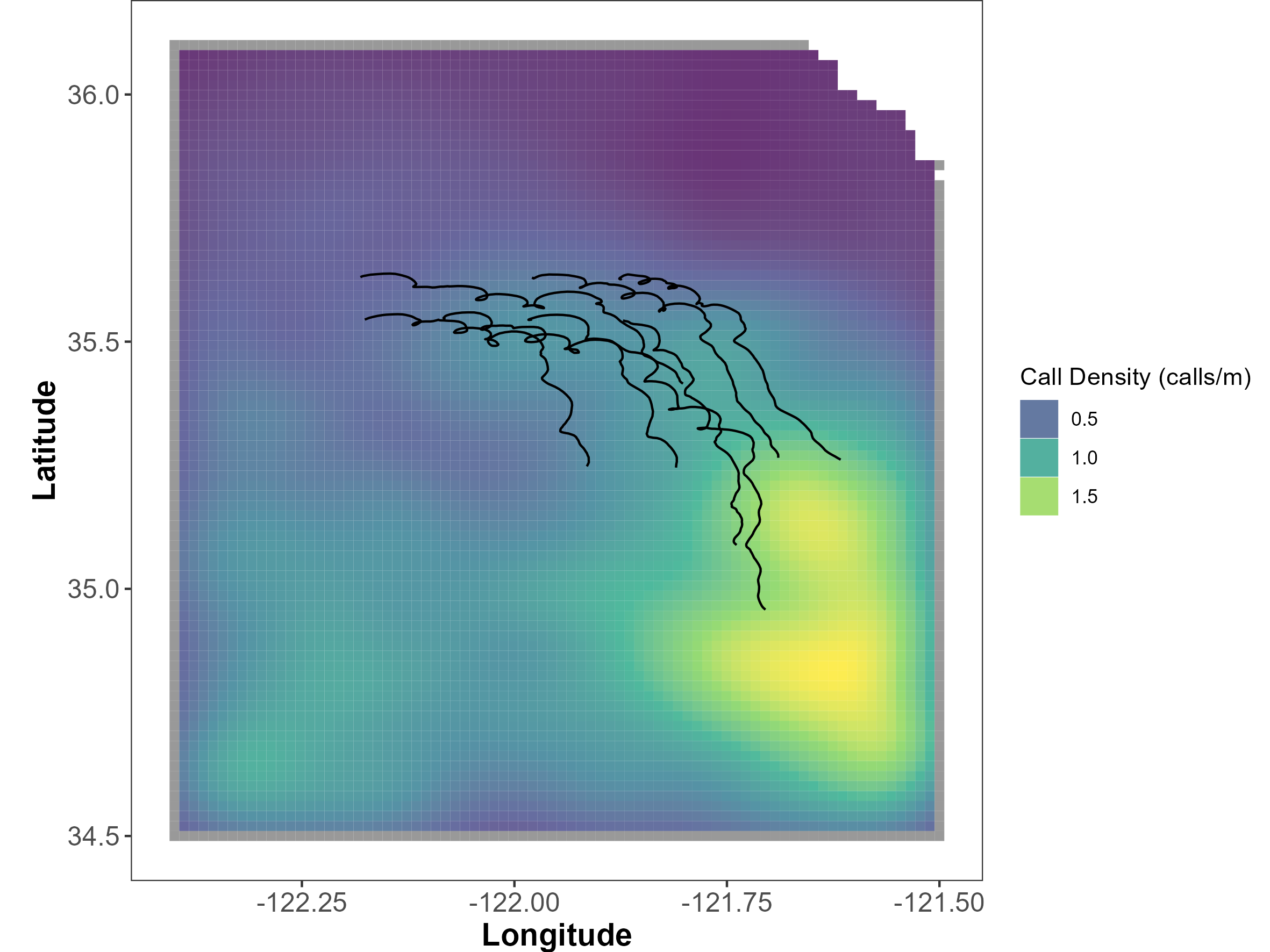
We simulated 4,000 calls distributed in the survey area according to predicted fin whale densities by (Becker et al. 2020) (Figure 1). We determined the minimum spatial resolution to which each call could potentially be localized using between 1 and 7 of the drifting recorders to compare the tradeoffs between localization resolution and the number of sensors.

Figure 1: Tracks of 8 clustered drifting recorders with simulated fin whale call density. Filled area represents simulated fin whale call density based on (Becker et al. 2020). Black lines indicate the drift path.

The proposed method is a grid approach that asks whether or not a call could have been produced by an animal in each of the grid cells within the survey region. The method involves two steps and accounts for spatial uncertainty throughout.

The first step in the localization method considers known biological parameters of the species and the measured SNR of the arriving call to determine the minimum and maximum range at which a call could have arrived.

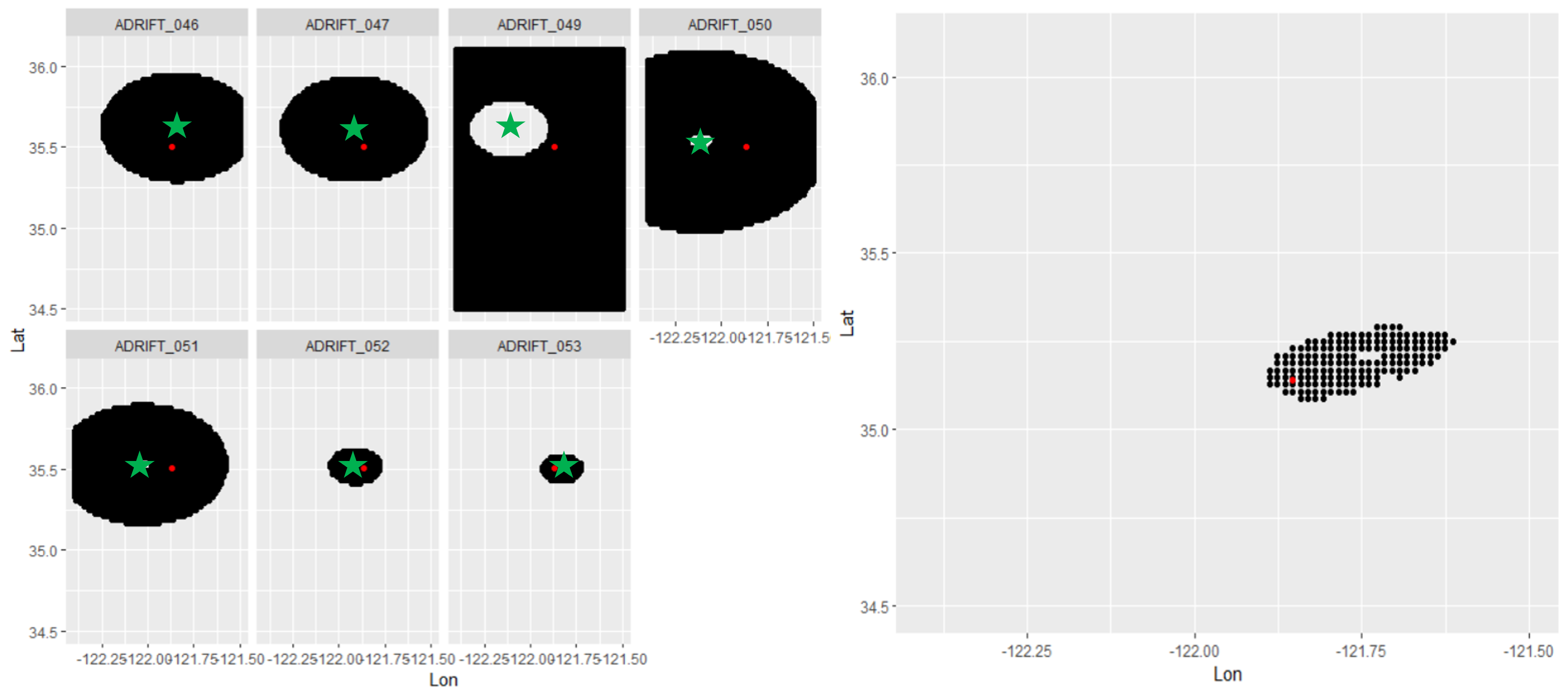
SNR is defined as the Source level of a call minus the noise level at the sensor and the transmission loss over the range between the source and sensor.[1] Thus, if a call arrives at a sensor with an SNR of 45 dB, the ambient noise level in the fin whale band was 120 dB, then we can use knowledge of source level distribution to estimate the minimum and maximum range of each call. If fin whale source levels range between 170 and 190 dB then we know the animal must have been 3.6 to 46.4 km from the receiver. Thus, an annulus (doughnut!) of potential call origin centered at each drifting recorder location is created for each call. This information is particularly informative by itself but with multiple drifting recorders the annuli can be overlapped to narrow down the region of origin (Figure 2).

The second step applies to calls that were detected on two or more drifting recorders. In this case, the time-difference-of arrival, with associated positional error, is used to further limit the region of origin established in the first step.

[1] https://github.com/JPalmerK/AmbiguityGrids

Figure 2: Variability in sound source location using multiple sensors. Potential location of a source (red point) as detected by each of the drifting recorders (green star) at a given point during the deployment. Black areas represent the region from which the call could have originated according to the arrival SNR at each drifting recorder. Note the call was not detected by Adrift-047 and as such only a minimum location is known (left). The potential region of origin for the call based on the intersection of all drifting recorders (right).

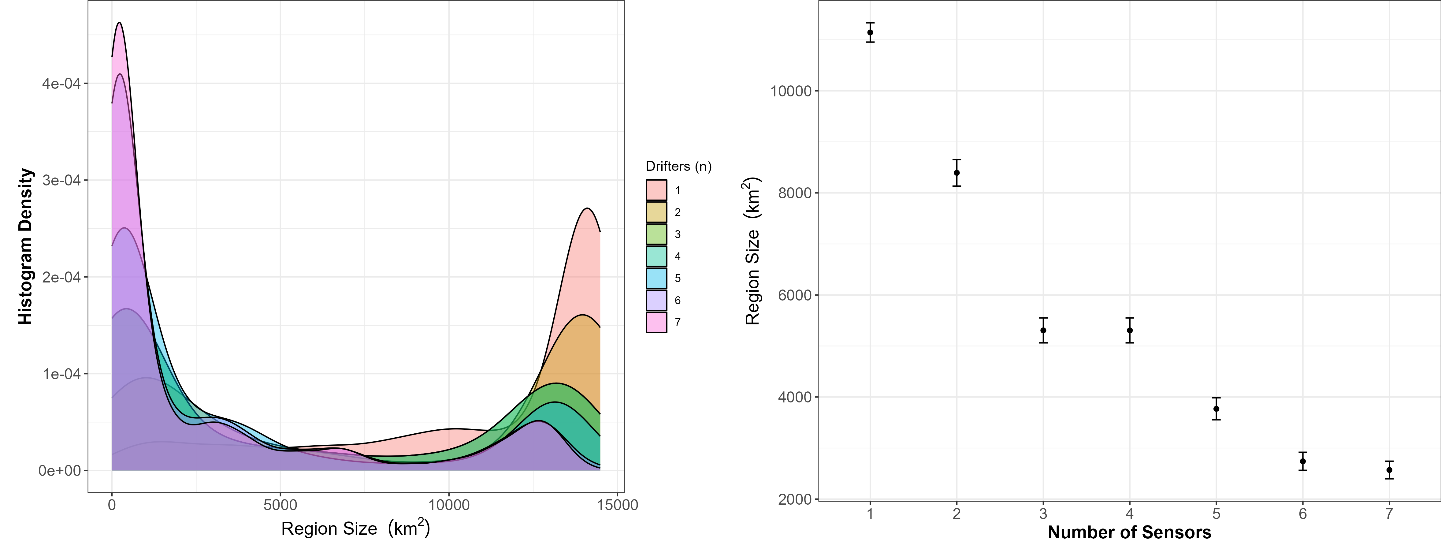
Using the above approach, we estimated the area associated with each region of origin produced from the calls in the simulation (4,000 calls). The histogram densities show a bi-modal distribution with a low region size associated with larger numbers of drifting recorders, and larger region size associated with lower numbers of drifting recorders (?@fig-Adrift_Appendix_HabitatMod_HistSpatialRes3). The scatterplot provides the mean and 95% confidence intervals of the regions of origin based on the number of sensors deployed in the array (Figure 3) The majority of the calls were in the southern portion of the survey area and calls in these regions could only be detected by one or two instruments at most.

Figure 3: Histogram densities and scatterplot of estimated sound source location size based on number of drifting recorders. Histogram densities (left) for the estimated total size of the sound source location for all calls in the simulation for different numbers of drifting recorders (shown as color). Scatterplot (right) of region size for different numbers of drifting recorders.

This preliminary modeling suggests that the dispersed sensors provided by the clustered deployment of multiple drifting recorders can allow for reducing the possible source location for sounds detected on multiple sensors. This improved spatial resolution of the sound source may improve the viability for using these data for population assessment.  Future research should test these analytical methods on real data such as those provided during the Morro Bay surveys and identify how these methods can be used for population assessment.